The Intersection-Jump Autorouter
I 100x'd my grid autorouter's performance using 3 iterative rules
The part 2 of this building autorouters series was supposed to be all about gridless autorouters and creating meshes to do autorouting, but while I was playing around with grid-based autorouters I discovered some interesting optimizations that blew the performance of everything I had done out of the water.
Why I was mad at grid-based autorouters
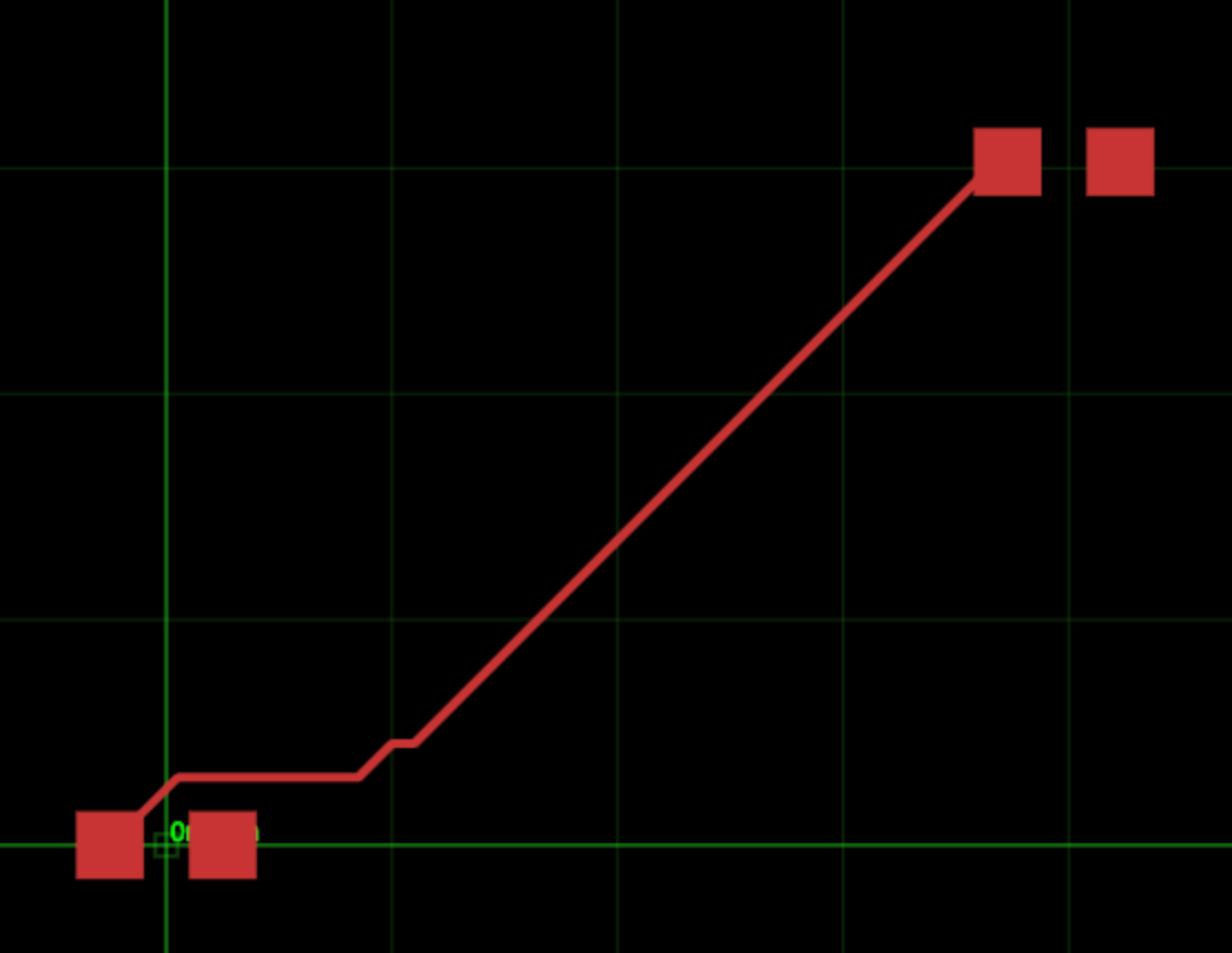
In Part 1 we built a grid-based autorouter and used the popular pathfinding.js library, but the simple-grid was extremely slow for the “distant-single-trace” dataset, which is basically just where there’s a ton of empty space. The reason it’s so slow is it’s doing a bazillion checks in wide-open space.
The benchmark showed that the simple-grid was extremely slow on "the “distant-single-trace” dataset, taking on average 70ms. Even the single-trace performance is a bit scary, taking 1ms for a single trace when circuit boards have thousands of traces completely dashes my dreams of having realtime-routed circuit boards.

Generating Navmeshes
Game engines will often throw out grid-based routing altogether and construct “navigation meshes” that contain all the points of interest for an autorouting problem.
I have a lot to say on navmeshes, there are so many techniques and interesting decisions, but I’m going to table that for now because there is one big problem with navmeshes- especially how they’re done in game development: they’re pre-computed. In a game, it’s totally okay to spend some time pre-computing meshes, even “baking them overnight”, but for circuit boards that are being edited in realtime AND have dynamic adjustments due to other traces being routed or adjusted, that precomputation step is just too expensive. I have a lot more to say on this, but I’ll save it for a future article!
Let’s talk about “infinite grid” autorouters
With the grid-based approach we worked on in Part 1, we iterated over each of our obstacles to compute a binary grid we would store in memory. Then you would know if there was an obstacle at a point by checking grid[x][y], but as I mentioned above, I don’t like pre-computation, so what if we defined a method isObstacleAt(x,y) that iterated over our obstacles and checked in realtime? Now we don’t have to precompute, and as a bonus we don’t need to pick a size of the grid!
Allow me to introduce the Infinite Grid Autorouter. To reduce the possibility of mistakes in the algorithm, I’m moved all the A* logic into it’s own class. To define our autorouter, we just have to tell it out to get it’s neighbors!
This algorithm has 3 basic steps:
Define the four directions we want to go in, left, up, right, and down. Each of these directions is represented with a vector (-1, 0), (0, 1), (1, 0) and (0, -1)
Filter any neighbors that are inside an obstacle
Compute the neighbors position by adding the direction vector to the current node
Concerned about iterating over every obstacle inside of
isObstacleAt? We’ll get to how we can do this efficiently using Quadtrees in a future article. It turns out this is a lot less important than the stuff I’m talking about today!
The critical insight: Optimal Neighbors = Massive Speedup
The neighbors above are computed just by moving one GRID_STEP in all four possible directions. For a 0.1mm step, this means it would take a hundred steps to traverse a distance of 10mm. With A* exploring out in multiple directions, this can multiply and waste thousands of iterations. There’s got to be a better way!
I don’t think I’ve completely cracked the egg on optimal neighbor selection, but I did find three heuristics that generate nearly optimal points for most cases. Follow the direction for a travelDistance until one of the following happens:
You hit a wall
You cross an axis that your goal is on
You overcome the obstacle that the parent node ran into
Heuristic 1: Hitting a wall
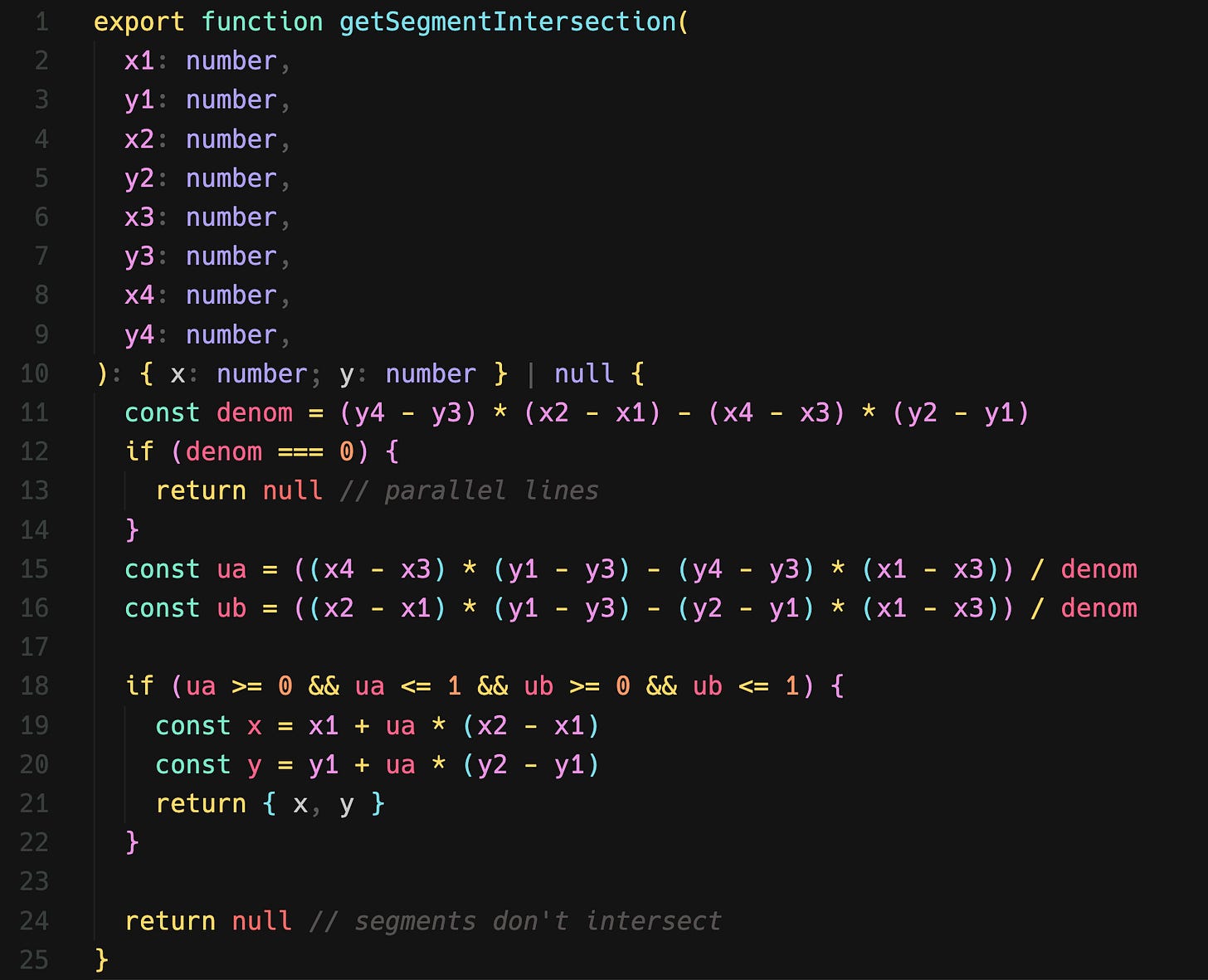
This is really simple, you just project the direction outward and compute when it intersects an obstacle.
Computing where two lines intersect is really fast, and rectangle obstacles are basically just 4 lines, so this is really easy!

Heuristic 2: Crossing the Goal Axis
Often times, there is no wall! We could travel on in a distance towards Infinity! To stop this, we add a heuristic where we stop along the “goal axis”, this means we’ll never pass by the goal without adding a new neighbor
Heuristic 3: Overcoming an Obstacle
This was definitely the most difficult heuristic to figure out, but it’s absolutely essential. With the Intersection Jump Autorouter we’re constantly running into walls, we want to place a neighbor whenever we hit a wall, change direction and overcome the wall. This allows us to “follow corners”
Let’s look at an example
The autorouting-dataset repo has a lot of tools for iterating over your autorouter to help you debug. Let’s walk step by step through an autorouting problem and look at the neighbors to understand how the IJump Autorouter works.
To get debug information/graphs, we just run
export DEBUG=autorouting-dataset*prior to runningbun startto start the development server.
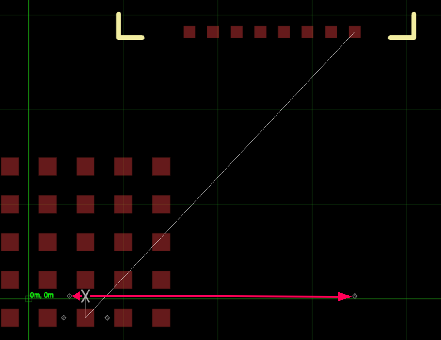
Let’s take a look at this problem, we want to connect the two squares connected by a white line.
Iteration 1: Hitting Walls on All Sides
In iteration 1, we hit walls on every side. Each neighbor is numbered by it’s position in the A* open set. 0 means your next up! Let’s see what happens.
Iteration 2: Passing the Goal Line
In this iteration, we explore to the right and left, because we’re blocked on an obstacle in the forward direction and we’re not allowed to backstep. The left neighbor goes until it overcomes the obstacle, the right neighbor goes until it crosses the goal axis.

Iteration 3: Going for Gold
The last iteration we go up until we pass the goal axis, which this time happens at the goal! We did it! Only 3 iterations!
That’s it?
Yes that’s it! Implementing this gives us a 100x+ speedup over our original grid-based autorouter, and no penalty for distant traces!
Comparing this to the simple grid-base autorouter benchmark, we have a clear winner!
Why is it so fast?
Where the simple-grid autorouter can take thousands of iterations, the ijump autorouter can take just 3-4. The main reason it’s better is it heuristics can be computed very quickly, and if the intersection is greater than 1 grid cell distance away, we’ve saved an iteration. In practice, this amounts to hundreds or thousands of iterations saved, making the cost of the intersection computation worth it.
It’s particularly good when the obstacles are sparse (like in the distant-trace dataset) but even with reasonably dense obstacles it tends to have many less iterations. The comparably low number of neighbors makes it easier for A* to select meaningfully different paths.
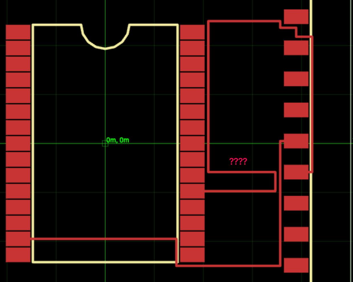
Where it fails
This autorouter is brand new, and I can’t find any literature on this technique (be sure to comment or message me on twitter if you find something), so there are a couple places where it doesn’t do so well.

Want to build an autorouter?
The autorouting-dataset (github) is a massive synthetic dataset of autorouting problems and a development environment for developing and benchmarking autorouters. I’d love to discuss and build autorouters together! There’s also a channel on our discord where I’d love to help :) I’d also love to sponsor contributors to work on autorouting algorithms!
All the code for the IJump Autorouter is available on Github here, you can view it against datasets online too!
We’re just getting started in our adventures building autorouters, subscribe if you’re interested, we’ve got multi-layer autorouters, navmeshes, and new datasets coming soon!


