Building a Grid-based PCB Autorouter
Build the best "getting started" autorouter, broken down step-by-step
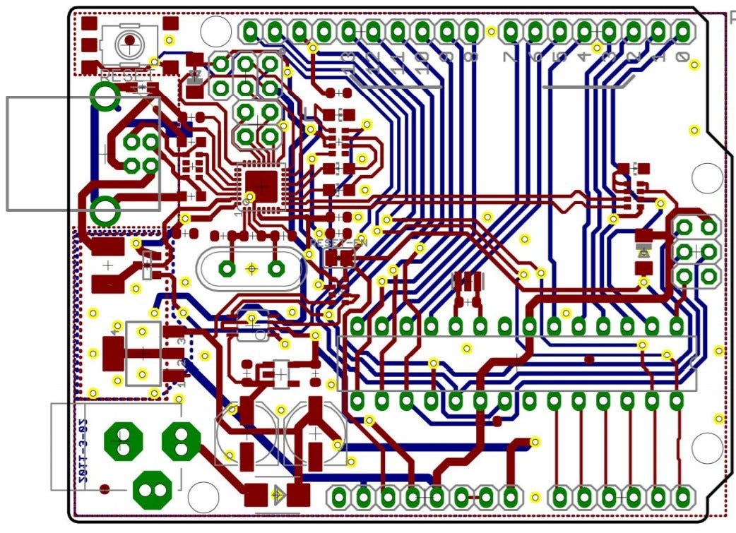
Autorouting is largely an unsolved problem. It’s the process of drawing all the little wires on a Printed Circuit Board that connect chips together. Believe it or not, this is still almost entirely done by humans today, people literally sit in front of a computer clicking and dragging to draw out each of the 1,000s of wires of a circuit. IMO it’s mostly unsolved because software engineers aren’t participating in the process of developing new autorouters, so in this post I hope to demystify some fundamental concepts.
Before you even THINK about nerd-sniping me with “actually, autorouting is a solved problem” - I know if you set up your constraints you can get decent results. The problem is even those results aren’t fast and people still can’t agree on what foundational algorithms are ideal. Once there’s an open-source solution with wide adoption and real usage we can call it a solved problem.
In this post, I’m going to show you how I quickly built the easiest of autorouters, a grid-based single layer autorouter. I’m also going to evaluate the autorouter on a new dataset of thousands of autorouting problems that you can play with or view online here.
This is Part 1 of the Building Autorouters Series where we’ll build different types of autorouters, Part 2 is about a gridless autorouting technique that uses line collisions, subscribe to stay tuned!
A quick note on terminology
For basic autorouting, you really only need to know a couple concepts
Chips are glued (soldered) to a circuit board by placing them on “Copper Pads”
To connect two chips together, we draw traces between their Pads
When drawing a trace, other Pads become Obstacles
That’s basically it! We’re just drawing lines.
Grid-Based Autorouting
Before we dive into the code (don't worry, it's coming), let's talk about why I chose a grid-based approach.
Pros of Grid-based Autorouting
It's Stupid Simple. Pathfinding on a 2d grid is incredibly common in game design, there’s almost certainly a library in your language that does it
Fast for dense “maze-like” designs without a lot of area
Consistent Clearance: Guaranteed clearance between traces. No awkward touching
Layer Friendly: Multi-layer routing? Just add more grids.
Cons of Grid-Based Autorouting
Limited Angles/Curves: Generally limits traces at 45 or 90 degrees (many EEs prefer this anyway)
Resolution: Sometimes, you need more cells than the grid allows, and increasing the number of cells increasing computation time.
Limited for Odd Pads: Funky pad shapes (and to a lesser extent circles) have trouble fitting onto a grid perfectly.
Performance limited by size of grid - your memory usage is going to scale with the area of your circuit board, this can be pretty intense since you’ll typically want to have each cell less than 0.1mm x 0.1mm
Let's Get This Party Started: Implementing Our Grid-Based Autorouter
Here's how we're going to structure this beast:
Grid Creation: We'll create our grid(s) based on the PCB dimensions.
Mark Cells with Obstacles Unwalkable: We'll mark all the components as no-go zones on our grid
Pathfinding and Routing: We'll set up our A* pathfinder and use it to route all our connections, avoiding any traces that have already been laid
All of the code we write today takes in “Simple Route JSON” and spits out JSON “pcb_trace” objects. In PCB land these simplified JSON formats are uncommon, most formats are in the form of s-expressions, deprecated XML files and hundred-page-spec binary formats.
Want to skip ahead? Here’s the source
Making the Grid
Let's construct a 2d binary grid with 0.1mm x 0.1mm cells.
Now we’ll set the inside of each obstacle as “unwalkable” by iterating over each obstacle, then each cell inside each obstacle’s bounds.
Pathfinding and Routing: Where the Magic Happens
Alright, this is where things get spicy. We're going to set up a A* pathfinder using the pathfinding module and use it to route all our connections.
For each connection, look at each pair of points (A & B) that make up the connection
Try to create a path from A to B using A*
If we find a path, add it to our array of pcbTraces
And there you have it! It's finding paths, laying down traces, and respecting the personal space of components.
This is basically the hello world of autorouters. For simple connections, it gets the job done, but as designs get more complex, you’ll want to implement algorithms on top of this like “rip and replace”, which is where you remove traces that are too often “in the way”. You’ll also notice that this autorouter is very order-dependent, the first trace is much more likely to get the shortest route.
The kryptonite of grid-based autorouters
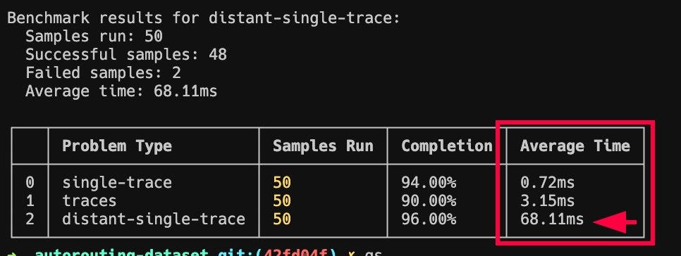
The performance of this grid solver falls apart as soon as you have traces separated by any distance. Creating a huge grid and checking for collisions all over it isn’t cheap! If you run this solver against the the distant-single-trace dataset, it suddenly becomes 94x slower, even though the complexity of the dataset in terms of pads and traces is identical to the single-trace dataset.
Running a benchmark using the npx autorouting-dataset benchmark confirms the slowness.
Conclusion- What’s Next
Grid-based autorouters definitely play their part, I think if you’re in a dense routing situation it can makes sense to whip out the grid, but we’re going to take a break from Grids in Part 2 and work on a totally different type of autorouter, one that uses line collisions and a BFS algorithm to quickly solve for autorouting paths regardless of the distance.
Can you think of what kinds of datasets stump a gridless autorouter? Want to make your own autorouter? Join the tscircuit discord, check out the Github, or subscribe to follow along!


