
Caching algorithms without knowing how they work
Everything worth computing is worth caching. Using vector similarity and synthetic problem generation to discover efficient hidden solution topologies

Here’s an interesting idea: You have an algorithm. It works but it’s slow. When you look at the solutions, you notice there’s commonality in a way that’s a bit difficult to describe. If the algorithm just knew it had solved a similar problem hundreds of times before, it could just recall that solution and “adapt” it a bit.
This is the situation we’re in with autorouting. We have a many similar solutions, but we don’t yet have a mechanism to retrieve those solutions and apply them to similar problems. More importantly, we don’t know how many of these solutions we would need to store to have something effective.
If you naively “cache” the exact coordinates of every pad, every hole and every required trace, you will find that you’ve stored terabytes of useless data- after all, every circuit board is unique and any slight change breaks the cache. If you store circuits lossy however, say by only storing the netlist and footprints, you’re likely to have a solution that is unusable as components are moved around.
So what do you store? How do you look up what you’ve stored? How do you apply it to a unique dataset?
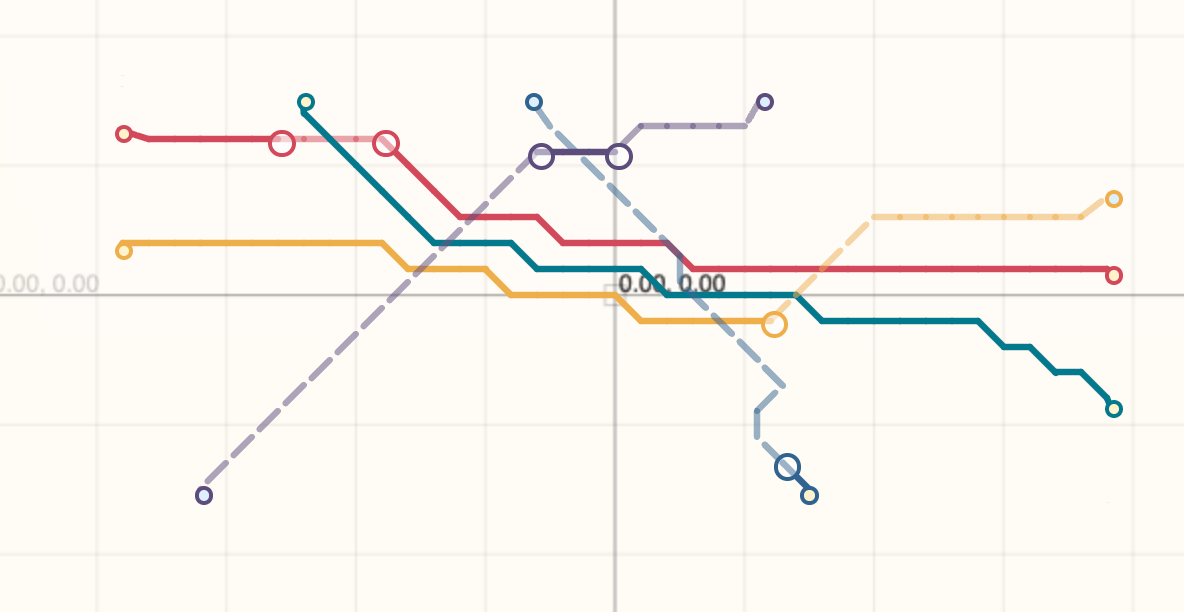
Our Case Study: Zero-Obstacle Autorouting
We’re going to study an approach to caching algorithms through the lens of the “zero-obstacle autorouting” problem, which is the most pure form of “the autorouting problem”. For the tscircuit autorouter, this is also the slowest phase of our autorouter and runs just after HyperGraph Autorouting. It is the algorithm that runs on “open space” in a PCB where there are no pads, holes or keepout obstacles.
Thinking of problems as vectors
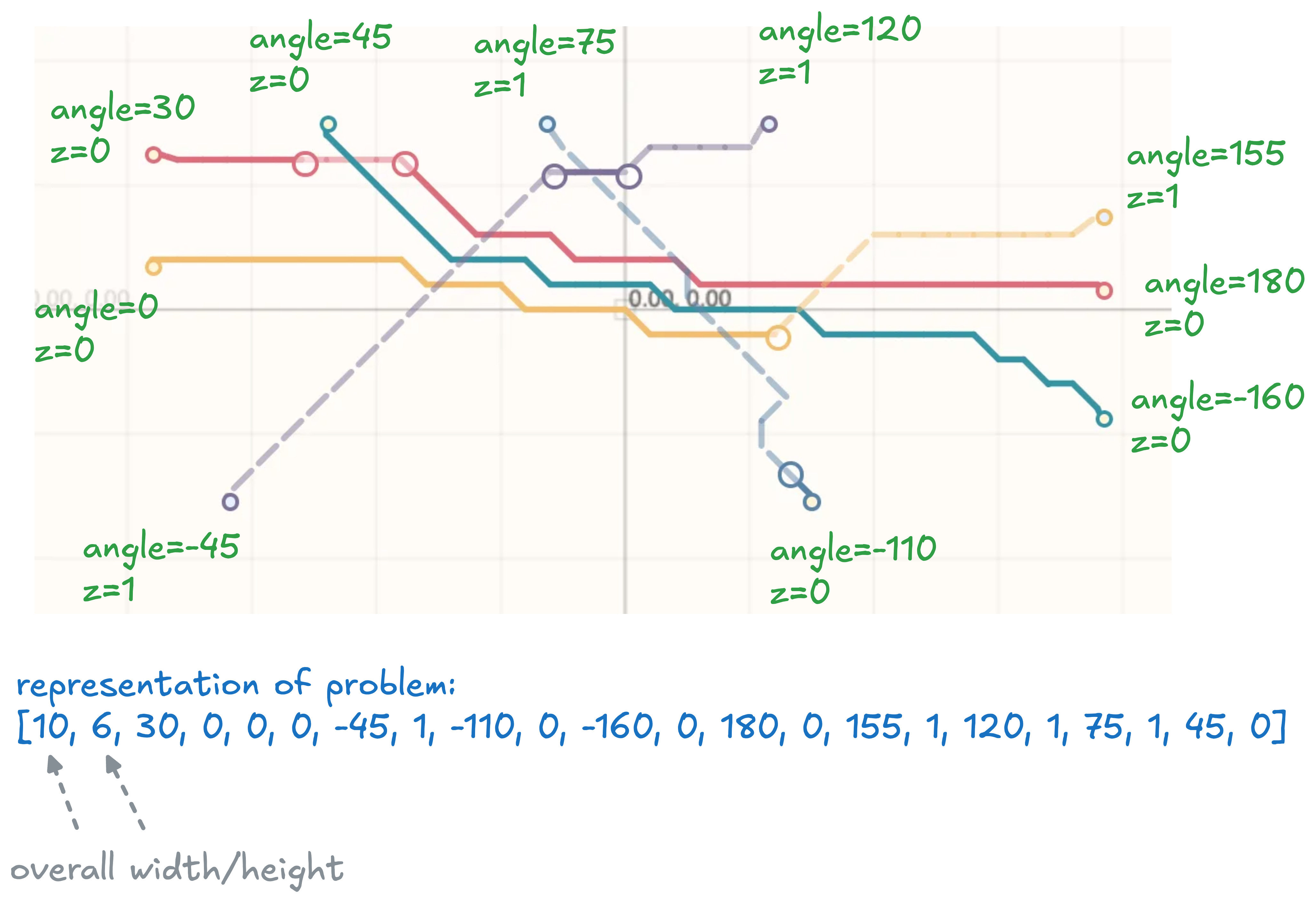
The first, most important problem to solve is the representation of the problem. Our problem representation gives us a clear insight into the “problem space”. The problem space is basically the number of unique problems that exist. In general, if you need more numbers or more data, the problem space is really big.
So let’s start by breaking down the problem into a vector, using as little data as possible. Sometimes to reduce the data representing a problem, you can “project” into a problem space that is more constrained. For example, instead of storing X and Y for each coordinate, we can just store the angle relative to the origin and the overall size of the problem. This great simplifies our representation of the problem, we now can represent each point of our problem with (angle, z) instead of (x,y,z)
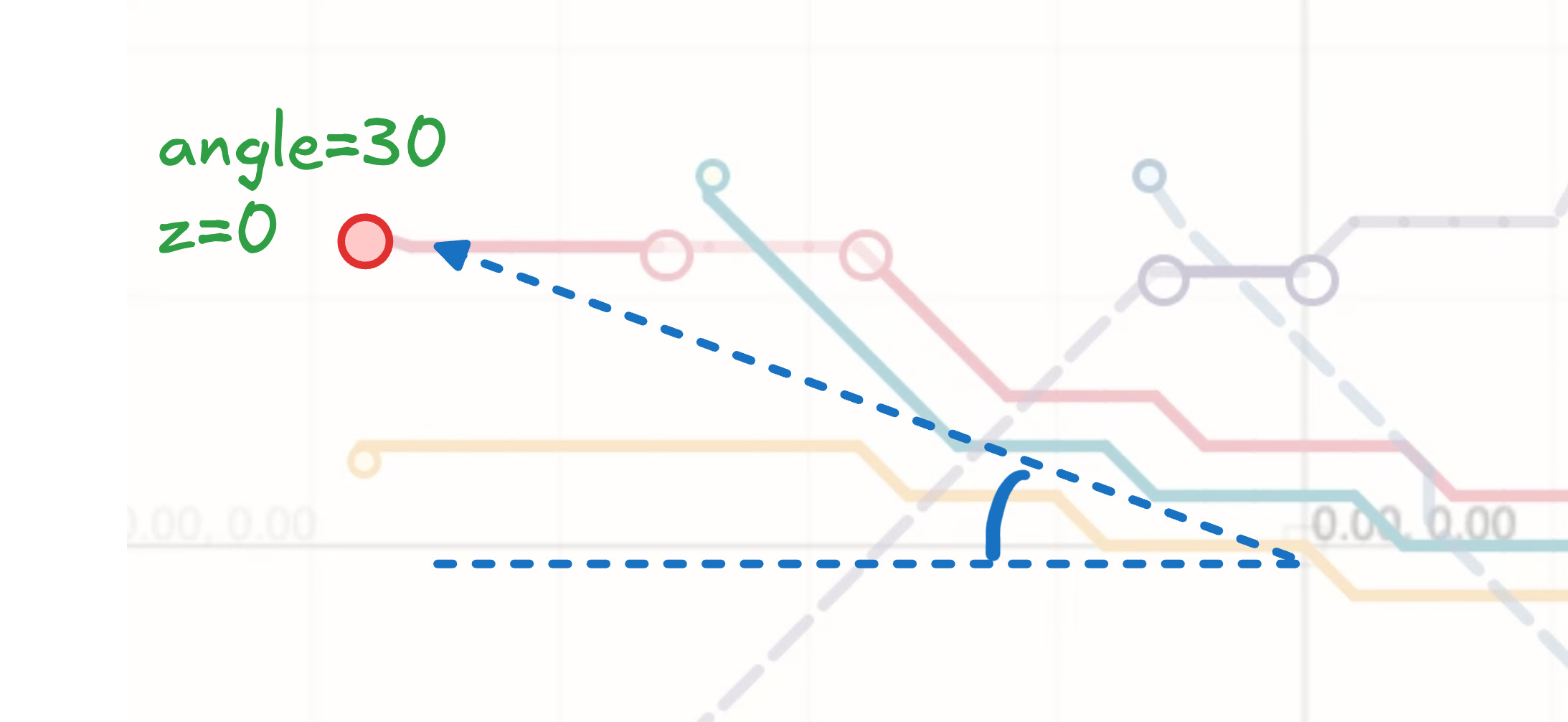
Trying to find ways to compress the problem space is a great exercise in exploring “what is actually important” for your problem. When we convert this problem into angles, we constrain the problem space. We can no longer handle points that have the same angle but are different distances from the origin- however, we never needed that problem space to begin with! We always organize points on the edge of a rect, so this is a GOOD constraint. If you can reduce the problem space to avoid invalid representations being possible, that is worth exploring!!
Vector Distance and Canonicalization
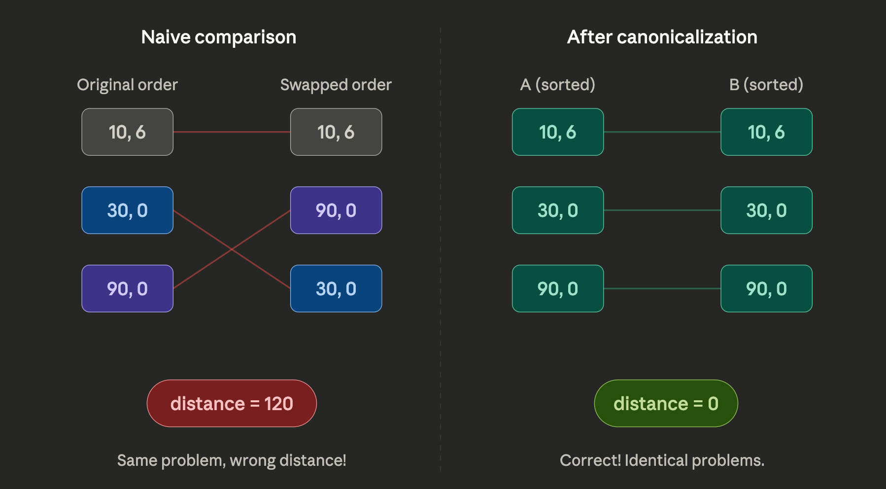
Now that we can think of our problems as vectors, it becomes possible to compute a “vector distance” between two problems. But before we get excited, we need to consider the type of similarity we’re interested in. We’re interested in a special kind of similarity, where two problems are similar only if they can share the same solution with some “tweaking”. We can’t just naively take the difference between each number in the vector and add up the differences, we have to find a more complex vector difference function that is tuned to return low distances for problems that can share a solution.
The “gotcha” of similarity functions in geometric spaces is you don’t really know if you’re comparing “apples to apples” when you’re comparing two parts of the vector. For our case-study, if we compare the two numbers in the array, we don’t know which two points we’re comparing. We might could have the exact same problem but with a totally different point order. The problems would appear to be very distant when we take the vector difference even though they share the exact same solution!
This is where the notion of “Geometric Canonicalization” comes in. This is where we sort or rearrange our vectors in a way that ensures we’re always comparing “apples to apples”. In our case, we can simple sort points by making the “lowest z, then lowest angles come first” Canonicalization can often create issues. For example in our case two angles may be very close together but sort such that they’re very far apart- like 0° and 359°. These issues can be mitigated elsewhere or absorbed into the size of the cache.
Ultimately, techniques like canonicalization and complex vector distance functions trade runtime for cache size. In our case, I knew we could reasonably handle 1 million entries in our cache, so we tuned our similarity functions and tweaking functions (which we’ll discuss below) until we had the runtime and cache-space tradeoff best for the autorouter.
Putting square pegs in square-ish holes (the “adapt” function)
When you have a “lossy” cache, you need to be able to pull a solution that may not be perfect and adapt it to the current problem. You can think of this as the “reverse cache transform” or the “adapt function”
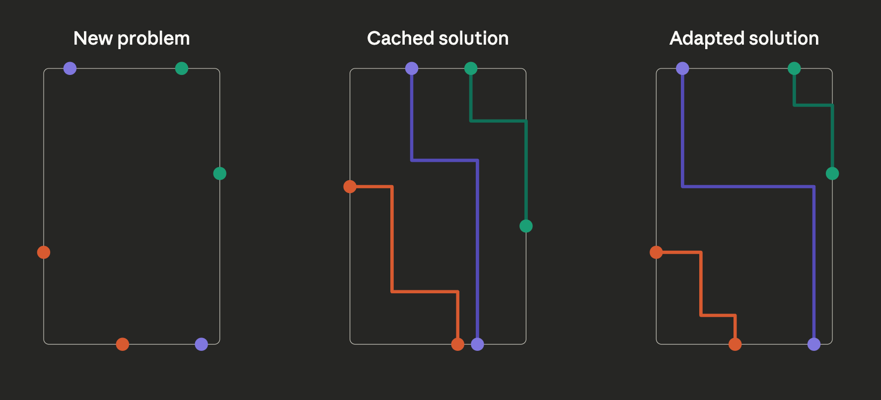
The reverse cache transform should execute quickly, because it is a runtime penalty. It should check and fail if it’s unable to adapt a solution, because this signals that a different cache entry should be used or generated. Later, we’ll use the adapt function to avoid populating our cache with entries that don’t improve the overall system accuracy.
Below, our “force-directed” adaption increases the “reusability” of cached entries by allowing them to tolerate shifting of problem points without DRC checks. This is a very simple and fast way to adapt a solution to a new problem.
Synthetic problem generation → Optimal Cache
For the zero-obstacle routing problem, we were able to generate a cache with 4,000 entries that can solve 99.9% of 4-trace problems. But to do this, we had to generate over 1 million synthetic problems to test on.
Because we don’t completely understand the underlying algorithm and what “hidden” solution topologies exist, we have to keep throwing random solutions at the cache to see what is solvable and what needs a new cache entry. After doing this for hours, we eventually start to see less and less DRC (design rule check) failures on our cache-adapted samples.
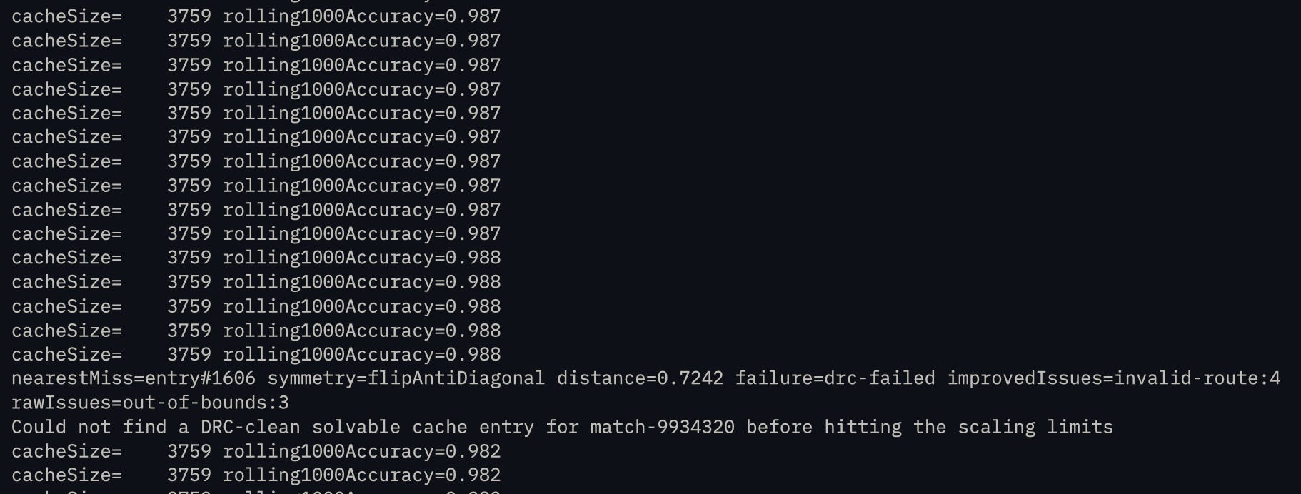
This is why synthetic datasets are so valuable. If solving a problem as simple as a 10x10mm square with 4 traces takes a million samples, then there isn’t enough human data in the world to tune an autorouting algorithm on a full board!
K-Nearest Neighbor, Shrink the cache for a slower runtime
The “Nearest Neighbor” is a super simple algorithm where you say “What data point is closest to the data point I’ve been presented with?” and return it. That is essentially what we’re doing- we measure what is “closest” with vector distance, and return the nearest solution. A well-known adaption to nearest neighbor is to take the K nearest neighbors instead of just the nearest neighbor. Each of these neighbors also “looks similar” to the problem at hand and is worth trying.
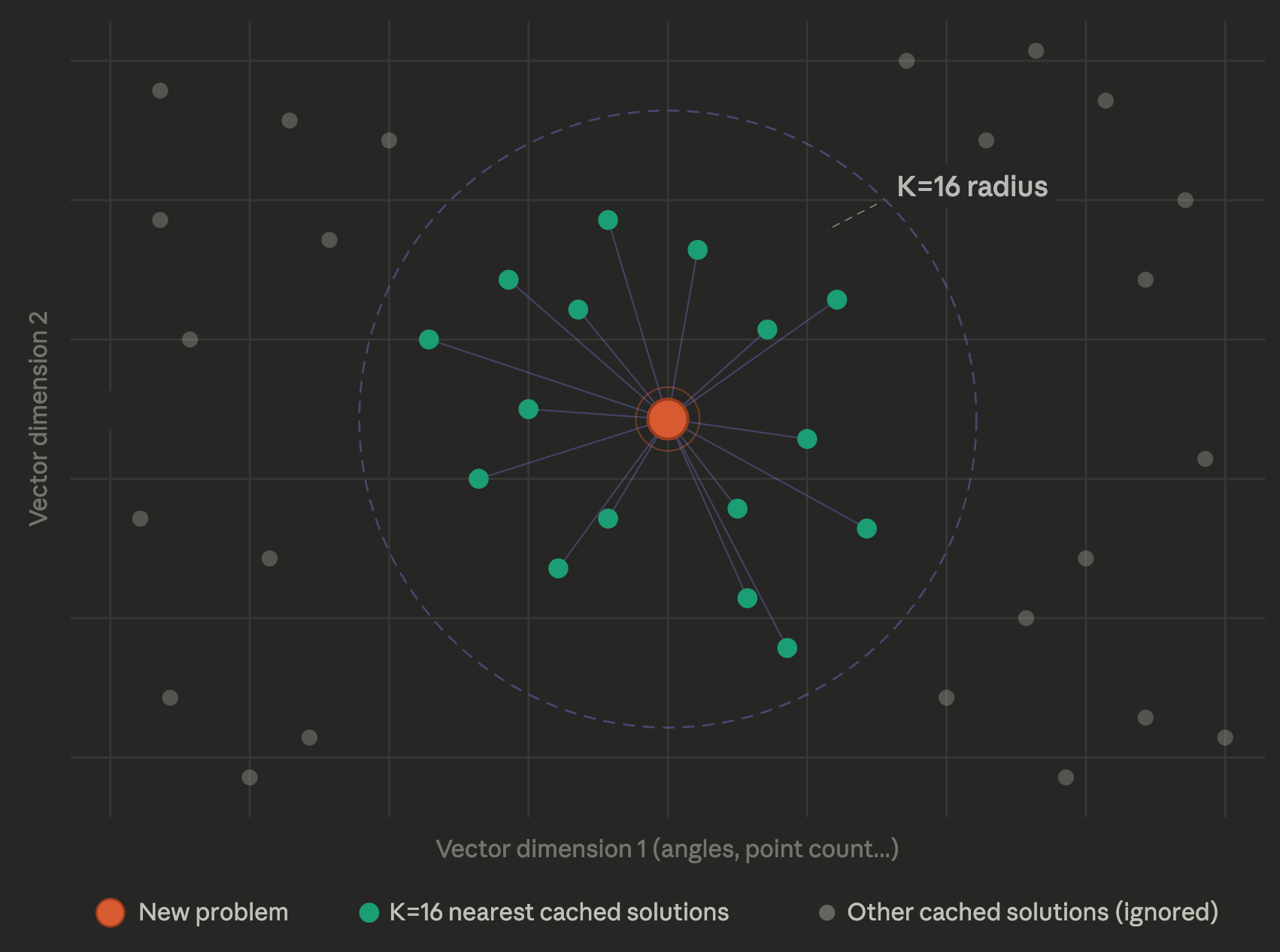
The benefit of K-nearest neighbor is you can get away with having a smaller cache and just pay higher runtime costs, since you have to adapt K neighbors instead of 1. In our case, we set K=16 because the runtime overhead didn’t cause much of a delay and our accuracy jumped up considerably with a smaller cache, making it so users can run the autorouter on their local machine. This is another knob to play with- sometimes storage is preferable, e.g. where you have a cloud machine backed by a massive KV store.
Exploit geometric symmetry (shrink the cache by 16x!)
The zero-obstacle routing problem has a lot of symmetry you can exploit. Symmetry means that a transformed version of the problem has the same solution, transformed. For example, negating all the X coordinates (flipping over the X axis) produces a problem that has the same solution just flipped over the X axis.
Each “axis of symmetry” halves the cache space you need to represent the problem. In our case, we can exploit this to reduce the cache size by 16x- meaning we only need to store 6% as many solutions in our cache. Here are the axes we exploit:
Rotating the problem by 90 degrees
Flipping over the X axis
Flipping over the Y Axis
Inverting the Z Layers (Top becomes bottom, bottom becomes top)
There are four ways to exploit symmetry:
Store all variants in the cache (reduce cache generation time)
Check all variants at runtime (reduce cache size, increase lookup cost)
Make vector distance functions understand symmetry (less conventional/supported vector lookup)
Canonicalize to a single variant (difficult to get right!)
Conclusion
This method of speeding up algorithm runtimes is fantastic because it adapts to any algorithm complexity. The framework of canonicalization, vector distance, and adaption greatly improves the efficacy of a cache and makes it possible to model complex geometric algorithms.
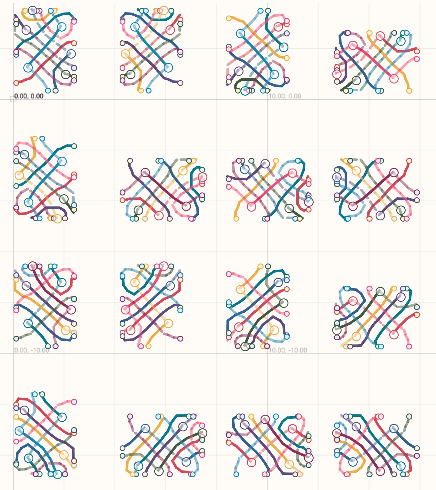
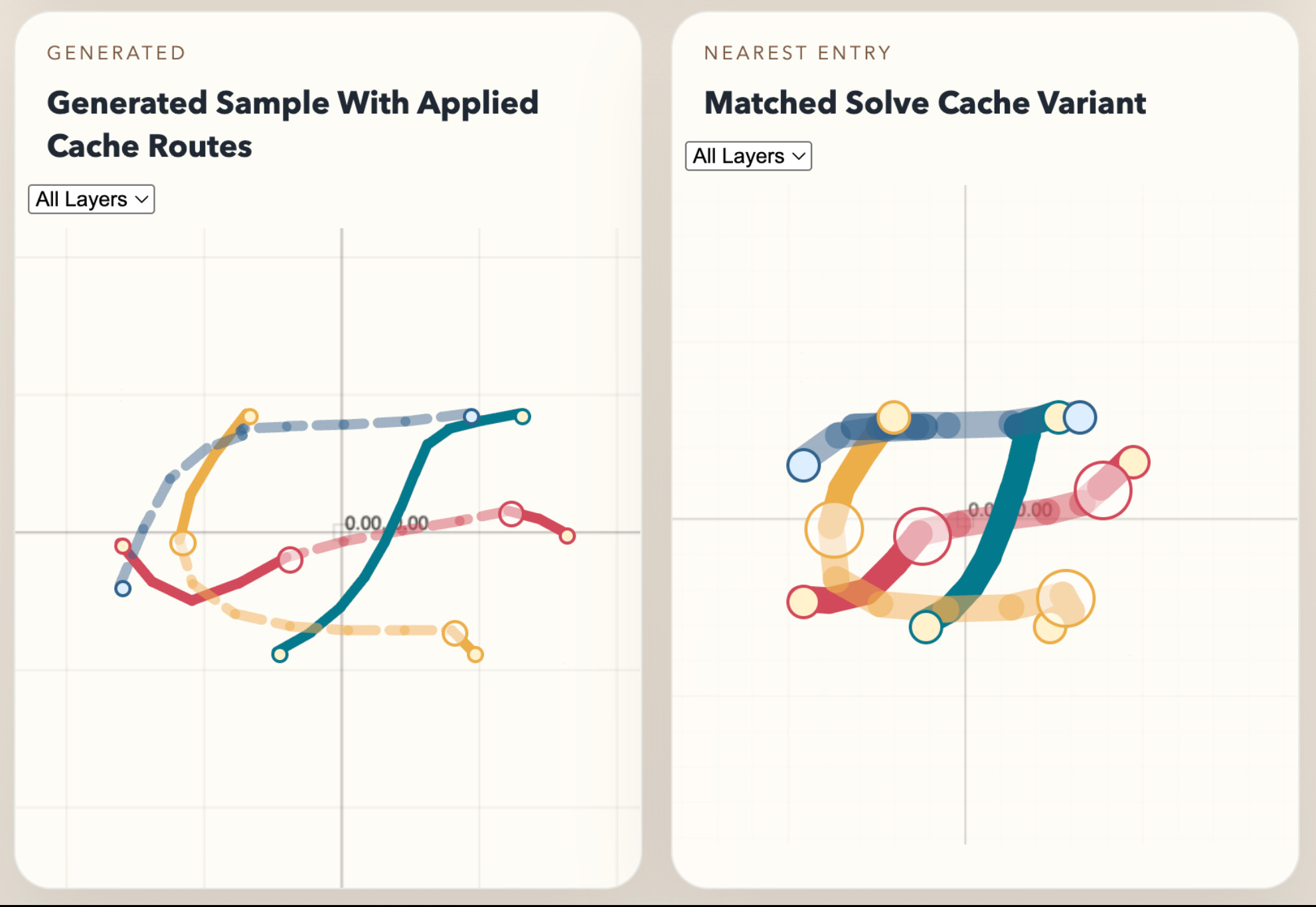
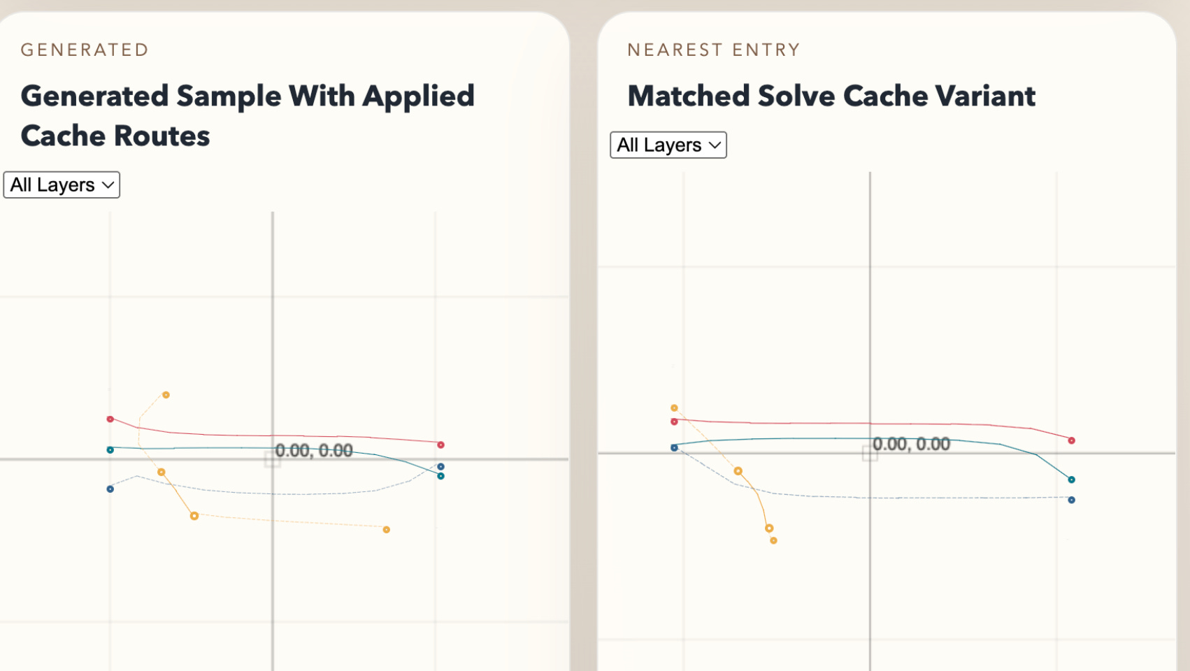
Here are some examples of our cache being used against generated problems:
If you’re interested in contributing to our autorouter or attempting some difficult algorithms, join the tscircuit discord or yell at me on twitter.