
HyperGraph Autorouting
The perfect datastructure for representing autorouting problems

HyperGraphs are a graph construction where in addition to edges and vertices you also have “regions”. These regions allow you to have more complex pathfinding functions that help with “global routing” of circuit boards by estimating the congestion of empty areas of the board. Hopefully by the end of this article I can convince you that this is the perfect primitive and methodology for PCB autorouting.

Why grid-based autorouters are ineffective
Normally when people think about autorouting, they think of grids and pathfinding. This simplification is why most autorouters can only route 50-100 traces then must give up or run for days to get a solution.
A grid creates an enormous solution space size. Because traces are very thin, the cell size of your grid must be 0.05mm or 0.1mm. Each of those cells can be “assigned” to any of your nets or marked as not-connected. Then you need to replicate the grid for each layer of the circuit board. For a modest 70x50mm 4-layer board, you’re looking at 280k cells with 50 possible assignments per cell. Or 50^280_000 possible states.
Now you might argue that not all of these states are possible (e.g. they are occupied by pads, keepouts etc.), but that’s precisely why the grid is a terrible data structure for an autorouter. Great data representations only represent valid states, and as a result the algorithms that operate on them are much simpler.
Enter HyperGraphs
Wikipedia defines HyperGraphs as follows:
In mathematics, a hypergraph is a generalization of a graph in which an edge can join any number of vertices. In contrast, in an ordinary graph, an edge connects exactly two vertices.
This wide definition is more than we need, let’s focus on a subset of HyperGraphs called “2-regular HyperGraphs”. These are HyperGraphs where each vertex belongs to 2 hyperedges (regions). With a bit of effort, we can convert any PCB routing problem into a 2-regular HyperGraph where the regions represent empty space, and the vertices represent available space on the edge of regions.
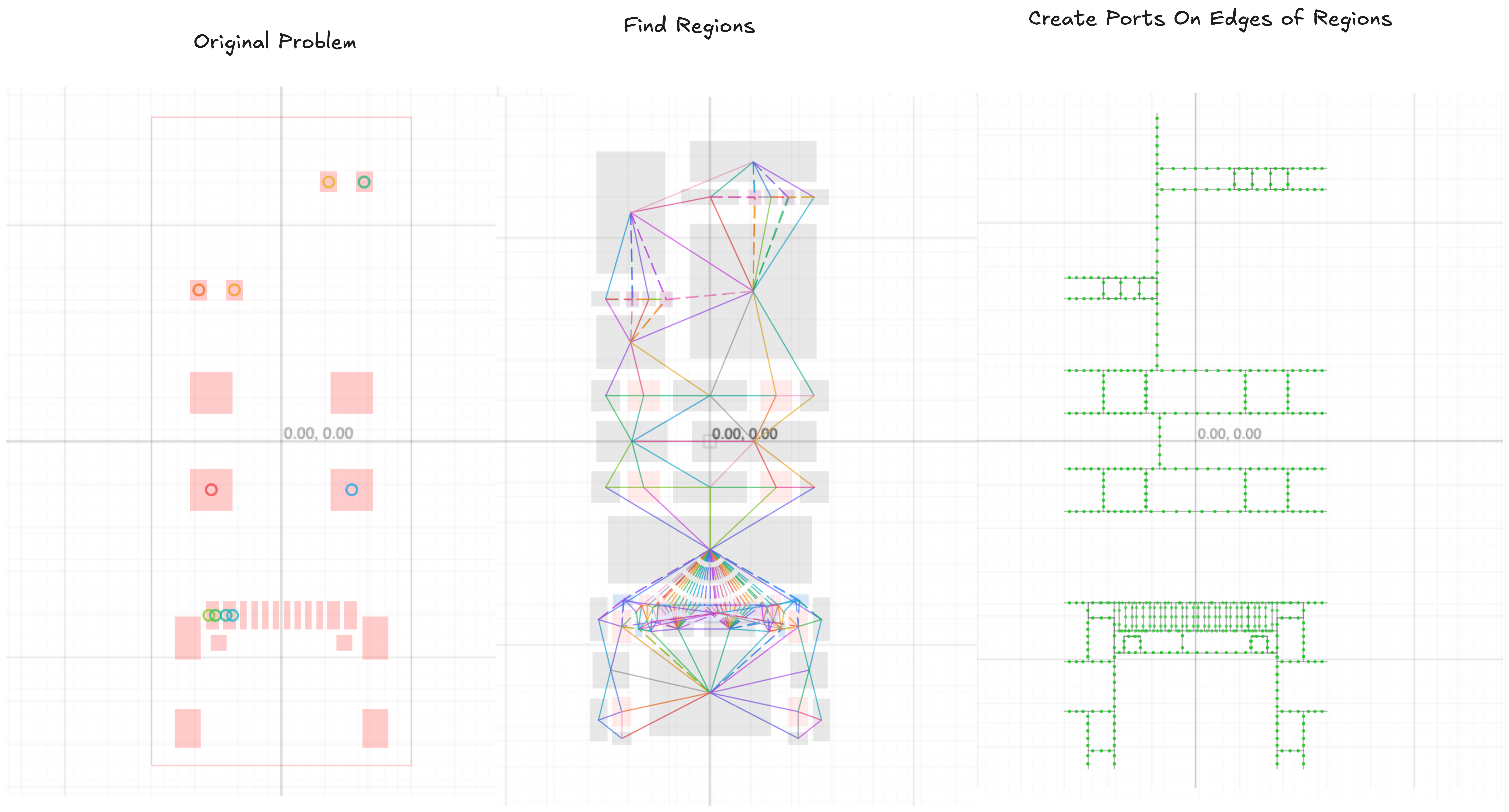
We can now route through a much smaller solution space, instead of routing over a grid that takes up this entire space, we can focus on only routing over relevant “bottlenecks” that relate to obstacles likes pads. This type of pathfinding is almost instantaneous, it only takes a few iterations to get across the board!
HyperGraph A*
So HyperGraph autorouters are really fast. But they don’t work quite the same as grid autorouters. In grid autorouters, doing an “occupancy check” is O(1), you simply ask “is there anything in the cell I want to move to?”. If there’s nothing there, that means you can explore it.
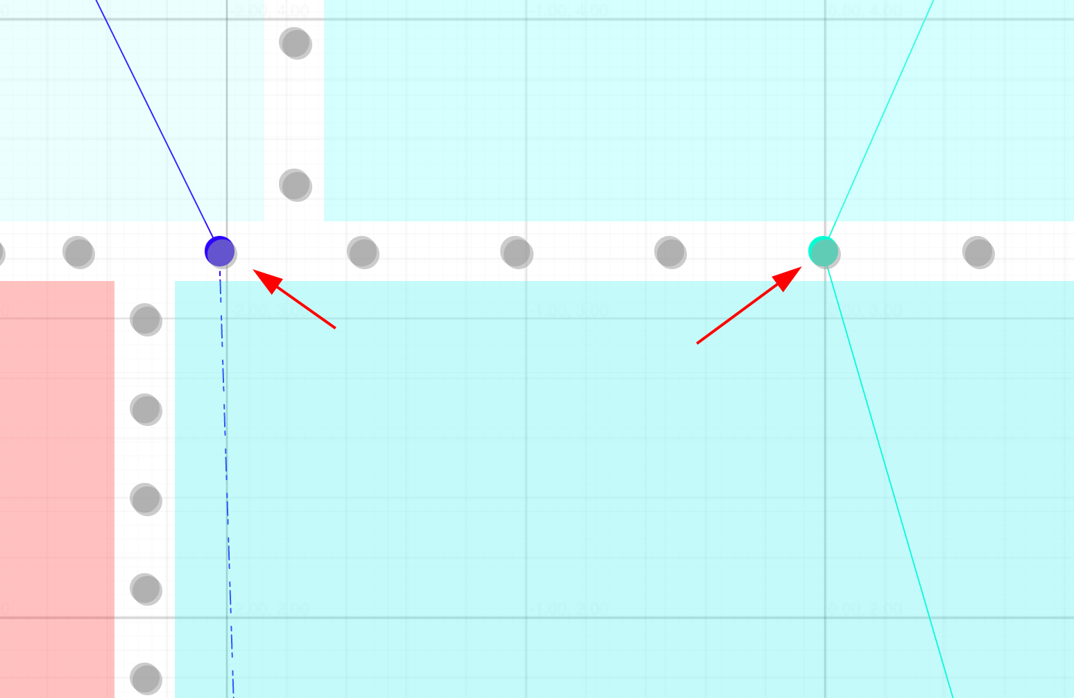
In HyperGraph Autorouting, you do something completely different. You use fast vector intersection math to check if moving through a port would trigger an intersection. This is the performance tradeoff, but it’s a good one. If your topology is set up well, you’re often not checking for intersections often, and when you do there’s only 1-2 traces to run intersection math on. Considering you can easily hop over 200 grid cells in a single iteration, this is much faster.
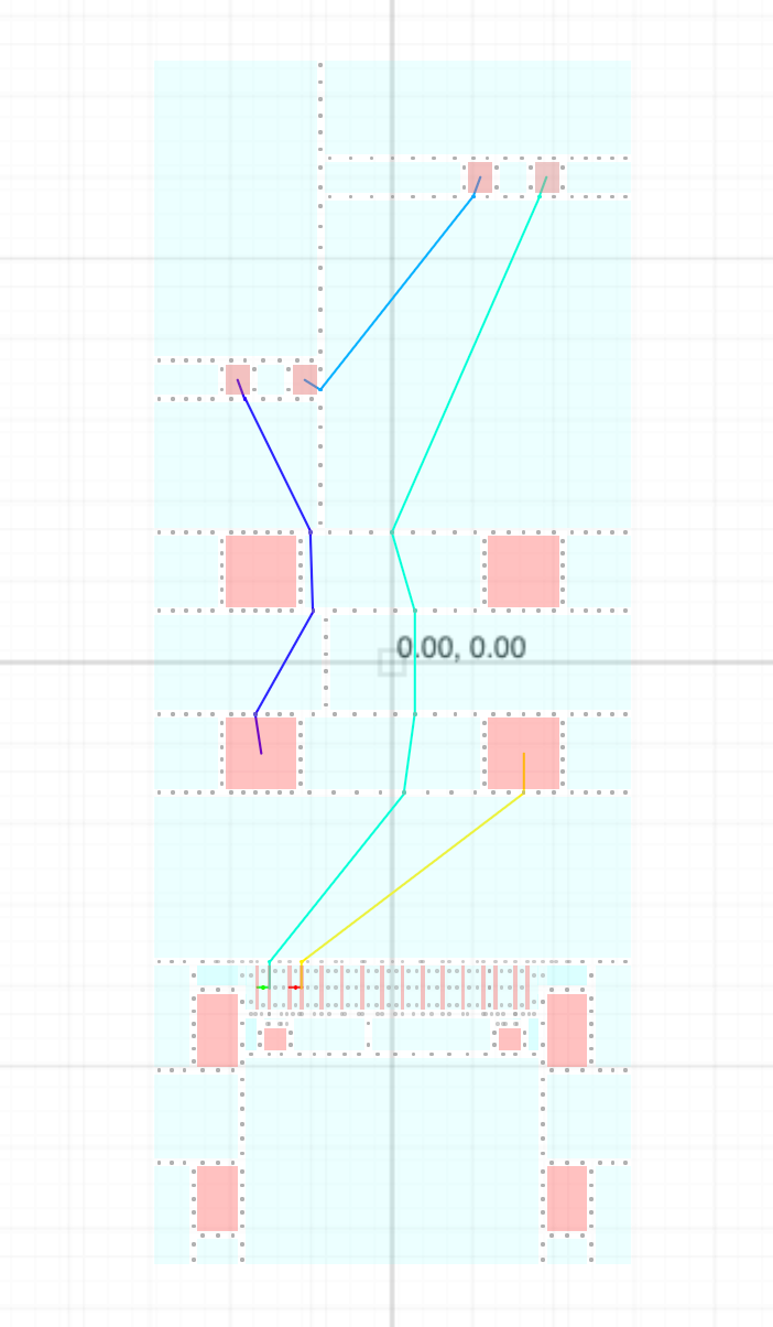
Here’s an animation of a HyperGraph autorouter solving how to connect 3 traces through 4 jumpers.
Handling Layers and Vias
HyperGraph regions, unlike grid cells, should occupy multiple layers. This can make the “topology construction”, the step where you generate the HyperGraph from pads and obstacles, very difficult (worthy of it’s own article). Every port is duplicated for each layer it could occupy, to represent all the different ways a trace could enter a region.
Now we’re in an interesting situation. It is actually possible for routes to “intersect” within a region because a via could be placed to make the crossing possible. Instead of not allowing crossings, we instead compute a “cost” for each crossing so that A* explores routes where intersections may take place.
Handling Zero-Obstacle Crossing Routes within a Region
So let’s say we’ve solved our HyperGraph, but we have crossing routes within our region. What do we do?
This type of problem is called the “zero-obstacle routing problem”. It is a beautifully simple problem. You have a rect, and you have pairs of points which you must connect without them touching using vias. There are no obstacles, and you can use any cell size that’s convenient. You can use a conventional grid based solver on this small region, or you can use vector-based methods. You can even combine solvers together. The zero-obstacle problem on rects with <20 traces is already known to be easy. We’ve successfully broken down the problem to a point where grid-based solvers are already known to work. In fact, you can have AI vibe-code you a decent zero-obstacle grid-based autorouter in couple minutes. Relative to full board solving, it is trivial!
Here’s a zero-obstacle A* grid-based solver in action, I got a bit impatient (there’s so much to explore!) but you can see even though it takes a lot of iterations, they’re particularly good for zero-obstacle problems and solve quickly (in clock time)
The perfect cost function for regions?
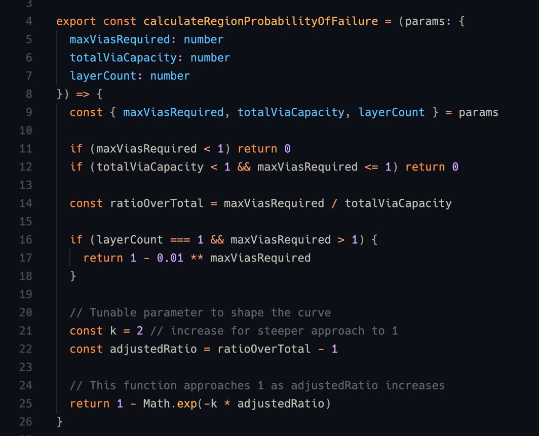
When you’re autorouting boards you can slowly build up a dataset of “high density zero-obstacle” problems, each of these problems may have zero-obstacle routing problems you could or couldn’t solve with your zero-obstacle router.
If you are clever, you can compose a cost function that predicts whether or not a region is solvable, then cost appropriately so that your “HyperGraph stage” heavily penalizes regions that are unlikely to be solvable with your zero-obstacle high density problem solver (usually a grid solver)
Conclusion
See it all come together:
HyperGraphs are an incredible and underutilized way to solve autorouting problems. If you’re interested in developing open-source autorouting algorithms with us please get in touch with me (seveibar) via our discord or contact@tscircuit.com
Want to see the code? Check out our state-of-the-art, lightening fast MIT-open-source autorouter!